Week 42: VaR and Risk Models — Parametric, Historical, Monte Carlo, and Why All Three Break in the Tails

---

1. Why This Is Important

Last week was the conceptual frame for risk management: position sizing, stop rules, scenario thinking, and how a portfolio's pain is budgeted across positions. This week we put numbers on it.

Value at Risk (VaR) is the single most-quoted risk number on the planet. Every bank, hedge fund, pension and insurance balance sheet runs a VaR system somewhere in its plumbing. **CVaR / Expected Shortfall** is its smarter cousin — required by Basel III since 2016 because plain VaR failed catastrophically in 2008. Both descend from the same idea: take a probability distribution of possible portfolio outcomes, look at how bad the bad days are, and quote a single dollar number.

You need to understand them for four reasons.

Common language. When a counterparty says "our 1-day 99% VaR

is forty million," that is a precise, falsifiable claim. If you cannot translate it into "they expect a loss of at least \$40m on one trading day in every hundred, and we have no idea how bad the worst one is," you cannot evaluate the statement.

Three calculation methods, three sets of lies. Parametric VaR

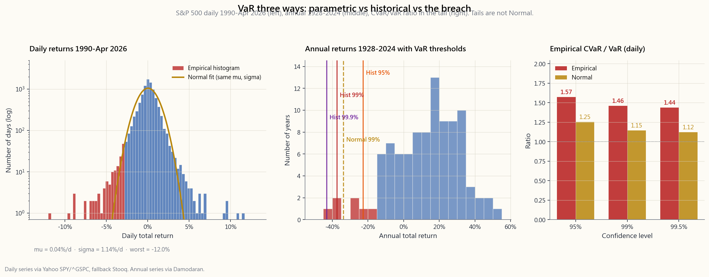
assumes returns are normal — which is wrong, especially in the tail. Historical VaR resamples the past — which only ever looked like the past you happened to draw from. Monte Carlo VaR makes you specify a model — and your model is a guess. The methods disagree most where it matters most: at the 99% and 99.9% percentile, and in the worst week of every decade.

The fat-tail problem. The kurtosis

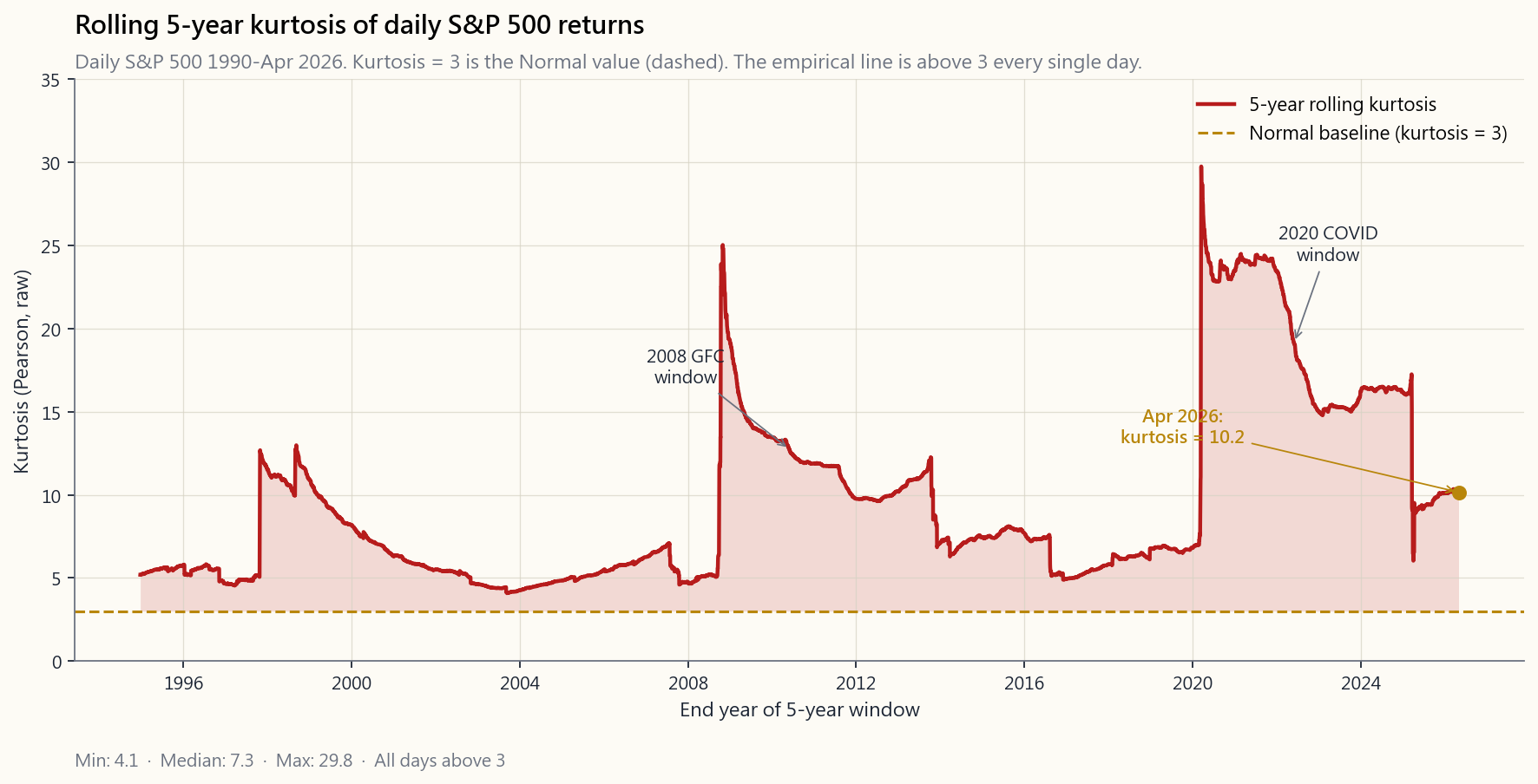
of daily US-equity returns runs 7-15 over 5-year windows since 1990, never close to the Normal value of 3. Parametric VaR at 95% underestimates real losses by ~10-30%. At 99% it underestimates by 2-5×. At 99.9% it is essentially science fiction.

CVaR is what regulators now use, and what you should use. The

Basel Committee replaced VaR with Expected Shortfall in the 2016 Fundamental Review of the Trading Book precisely because CVaR averages the whole tail rather than reading one point on the distribution. It is more conservative, harder to game, and coherent in a mathematical sense VaR is not.

The marshmallow conclusion at the end of this lesson: *parametric VaR is fine at 95%, useless at 99.9%, and the difference between the two ate Long-Term Capital Management in 1998, the structured-credit desks in 2008, and the leveraged vol-targeters in March 2020.*

---

2. What You Need to Know

2.1 The Definition — One Sentence, Three Parameters

Value at Risk is the **largest loss not exceeded with a given probability over a given horizon**. Three parameters, always:

Confidence level $\alpha$. Typical values: 95%, 99%, 99.5%,

99.9%. The complement $1-\alpha$ is the tail probability we are measuring — at 99% we are looking at the worst 1% of outcomes.

Time horizon $T$. Typical values: 1 day, 10 days, 1 month, 1

year. Bank trading desks use 1-day. Basel uses 10-day. Asset allocators use 1-month or 1-year.

Currency amount. The VaR number itself, in dollars.

The textbook sentence:

1-day 99% VaR = \$5,000,000 means: on 99 trading days out of every 100, we expect the portfolio to lose less than \$5,000,000 over a single day. On the remaining 1 day, the loss may be larger — and VaR is silent on how much larger.

That last clause is the big one. VaR tells you the threshold of the loss that will be exceeded $1-\alpha$ of the time. It tells you nothing whatsoever about how bad the breach will be when it comes. Two portfolios can have identical 99% VaRs and wildly different 99.9% VaRs — one capped at -\$10m, the other unbounded.

2.2 Method 1 — Parametric (Variance-Covariance)

The fastest, oldest, and most often wrong method. Assume daily returns are Normal with mean $\mu$ and standard deviation $\sigma$. Then the VaR at confidence level $\alpha$ over horizon $T$ is:

$$ \text{VaR}_\alpha = -\big(\mu T - z_\alpha \,\sigma\sqrt{T}\big)\,V $$

where $V$ is the portfolio value and $z_\alpha$ is the standard Normal quantile. The classic $z$ values:

$\alpha$	$z_\alpha$	Tail prob.
90%	1.282	10%
95%	1.645	5%
97.5%	1.960	2.5%
99%	2.326	1%
99.5%	2.576	0.5%
99.9%	3.090	0.1%
99.99%	3.719	0.01%

Plug in the S&P 500 daily numbers: $\mu \approx 0.04\%$ per day, $\sigma \approx 1.1\%$ per day. On a \$1,000,000 portfolio:

• 1-day 95% VaR: $-(0.0004 - 1.645 \times 0.011) \times 1{,}000{,}000 \approx \$17{,}700$.
• 1-day 99% VaR: $\approx \$25{,}200$.
• 1-day 99.9% VaR: $\approx \$33{,}600$.

These are the numbers a bank's 1990s spreadsheet would have spit out. Now look at what actually happened: October 19th 1987 the S&P 500 fell 20.5% in a single day. Under the parametric model that is a $z = 19$ event — its probability is $10^{-79}$, which is to say *it should not happen between now and the heat death of the universe*. It happened. On a Monday. With Reagan in the White House.

That single observation is enough to tell you the model is wrong.

The strength of parametric VaR: it is fast, additive, and easy to push through a portfolio with thousands of positions. Variance adds, correlations are linear, you can compute it in a spreadsheet.

The weakness: $\sigma$ is computed on quiet windows and then used to predict noisy ones, and the Normal distribution has thin tails that nobody's portfolio has ever seen. *At 95% it is an estimate. At 99% it is a guess. At 99.9% it is fiction.*

2.3 Method 2 — Historical Simulation

Drop the Normal assumption entirely. Take the last $N$ days of portfolio returns (typically 250 to 1,000 trading days), sort them, and read the empirical $1-\alpha$ percentile directly off the sorted list. If $N=1000$ and $\alpha=99\%$, your 99% VaR is the 10th worst return in the sample.

Worked example. Take SPY's last 1,000 trading days, sort, the 10th worst is roughly $-3.6\%$. On a \$1m portfolio, 1-day 99% historical VaR is \$36,000 — roughly 40% larger than the parametric number above. The history "knows" about COVID, knows about 2018 Q4 vol, and weights those days equally with quiet ones.

The strength: makes no parametric assumption. If the past has fat tails, your VaR has fat tails for free.

The weakness: you only see what happened. If your 1,000-day window ends in October 2007, you have no 2008 in your data and your 99% VaR will read like 95% the moment the regime breaks. The window is either too short (unstable, no tails) or too long (mixing regimes that no longer apply).

The cure is partial: age-weighted bootstrap (recent days count more) or filtered historical simulation (rescale yesterday's returns to today's volatility). Both push the model toward what a practitioner already does intuitively when looking at a chart.

2.4 Method 3 — Monte Carlo Simulation

Specify a model. Simulate $M$ paths from it. Compute portfolio P&L for each path. Sort. Read percentile.

The model can be Normal (in which case Monte Carlo agrees with parametric, with sampling noise). Or it can be Student-t with low degrees of freedom (heavier tails). Or a regime-switching mixture (quiet days from one Normal, noisy days from another). Or GARCH (volatility today depends on volatility yesterday). Or a jump- diffusion (Normal noise plus occasional Poisson jumps).

The flexibility is total. A typical "modern" Monte Carlo for daily US-equity portfolios uses a Student-t with 5-7 degrees of freedom — producing tails that approximately match the empirical distribution. This is the model bank-prop desks adopted after 2008.

Strength: can capture nonlinearities (options, structured products), path-dependent payoffs (barriers, callables), and any non-Normal distribution you can write down.

Weakness: garbage in, garbage out. If your model is wrong in the tail, your Monte Carlo VaR is wrong in the tail — with the illusion of precision. Running 100,000 paths from a wrong model gives you a confidently wrong answer.

The honest practitioner runs all three methods side by side, treats the spread between them as the irreducible uncertainty in the number, and reports the most conservative (largest) one.

2.5 CVaR / Expected Shortfall — The Average of the Tail

CVaR (also called Expected Shortfall, ES) answers the question VaR ducks: *given that the loss has exceeded the VaR threshold, what is the average loss?*

$$ \text{CVaR}_\alpha = \mathbb{E}[L \mid L \geq \text{VaR}_\alpha] $$

For a Normal distribution and continuous loss $L$, CVaR has a closed form:

$$ \text{CVaR}_\alpha = \mu + \sigma\,\frac{\phi(z_\alpha)}{1-\alpha} $$

where $\phi$ is the Normal PDF. The ratio $\text{CVaR}/\text{VaR}$ under the Normal model is roughly 1.25 at 95% and 1.15 at 99% — meaning the average breach loss is only 15-25% bigger than the VaR threshold under the assumption of Normality. Empirically on US equities the ratio is closer to 1.30-1.50, especially at the 99%+ levels. Tails are not just fatter than the Normal predicts; the depth of breach is also larger.

CVaR is coherent (in the formal sense of Artzner-Delbaen-Eber- Heath, 1999) — meaning it satisfies four properties any reasonable risk measure should: monotonicity, sub-additivity, positive homogeneity, and translation invariance. VaR is not coherent — it fails sub-additivity for heavy-tailed distributions, meaning the VaR of two portfolios combined can be larger than the sum of their individual VaRs. That mathematical pathology has practical consequences: VaR can incentivise hidden tail-risk concentration that CVaR penalises. Basel III replaced VaR with ES at the 97.5% level for exactly this reason.

2.6 Why All Three Methods Break in the Tails

The fundamental problem is summarised in one number: kurtosis.

A Normal distribution has kurtosis exactly 3 (or excess kurtosis zero). Higher kurtosis means fatter tails — more probability mass beyond ±3σ than the Normal allows.

What does the data say? Compute rolling 5-year kurtosis on daily S&P 500 returns since 1990 and the answer is: never close to 3. Mostly between 7 and 15. The 1987-window prints above 30. The 2008-window prints around 12. Even quiet windows like 2003-2007 print around 5.

The implications for VaR:

• At 95%: parametric VaR underestimates by 5-15%. Tolerable.
• At 99%: parametric VaR underestimates by 30-100%. Material.
• At 99.9%: parametric VaR underestimates by 2-5×. Useless.
• At 99.99%: parametric VaR is a polite fiction.

The 1998 LTCM blow-up was not a 1-in-a-million event under the fund's model; it was, in retrospect, a reasonably common 1-in-50- years scenario that the model could not see. The 2008 mortgage-bond losses were "twenty-five-sigma events, several days in a row" said Goldman's then-CFO David Viniar — which is a confession that the model was the wrong shape, not that the world was. March 2020 saw SPY trade -12% in a single session against a parametric model that assigned that move a probability of ~$10^{-25}$.

The right lesson is not "use a more complicated VaR." The right lesson is *risk numbers are estimates, all of them, and the tail is where estimates lie hardest*. The tail wags the dog. Your risk system must include explicit stress tests at multiples of the quantitative VaR, regardless of what the model says is "impossible."

2.7 Putting It All Together — A Practical Framework

How a serious investor uses these tools:

Run all three methods. Parametric, historical, Monte Carlo (a

Student-t with df=5-7 is the standard choice). Look at the spread.

Quote CVaR, not VaR. The 97.5% CVaR is roughly equivalent to

the 99% VaR for thin-tailed distributions and substantially more conservative for thick-tailed ones. Basel uses 97.5% CVaR; you should too.

Always run a stress test. Compute the loss under: 1987 (-22%

in a day), 2008 (-9% in a day, -38% in a year), 2020 March (-12% in a day, -34% in a month), 2022 (paired bond+stock drawdown). These are not VaR events; these are plan-for-them events.

Size positions for the tail, not the average. Run a

barbell. Most of the book in defensive holdings sized for normal vol; a small high-conviction tail in instruments that cap your loss (long options, deep cash buffers, defined-risk spreads).

Discount the headline number. Whatever VaR your platform

reports at 99%, double it for sleep purposes. The cost of being too conservative is a few basis points of opportunity. The cost of being too aggressive is the obituary section of the *Wall Street Journal*.

**Horace's view — VaR is institutional theatre, and the retail fix is structural, not statistical.** My own read of these models, after watching them fail in 1998, 2008, and March 2020, is that VaR exists primarily because regulators and risk committees need a single number to put on a slide. It is theatre. It systematically under-reports exactly the regimes where you actually need a risk number — the vol-on tail expansions, the regime turns from compression to expansion, the days when the option tail wagging the equity dog produces moves the model says are impossible. Kurtosis of 7 to 15 versus the assumed 3 is not a small calibration issue; it is the model being the wrong shape. The big banks discovered this in tears, every cycle, and the response is always to add another bell and whistle to the model rather than admit the model class is wrong.

The retail answer is not a better VaR. It is a better *portfolio shape*. I run a barbell with a small persistent long-volatility and tail-hedge sleeve sized so the worst-case loss on the hedged book is the known premium I pay for the hedge — not a model output that lies in the tail. The asymmetry sleeve is bounded by structure (long options, defined-risk spreads, deep cash buffers) so the CVaR on the worst week is a number I chose at position-sizing time, not a number a Student-t tells me after the fact. That is the inversion: instead of computing risk on a portfolio shape that has none, choose a portfolio shape whose worst case is bounded *by construction*, and let the VaR number be a sanity check rather than the load-bearing input.

---

3. Common Misconceptions

"99% VaR means the worst loss is bounded by VaR." No. 99%

VaR is the threshold beyond which 1% of outcomes lie. It says nothing about how far beyond. The worst-case loss is unbounded.

"A higher confidence level is always more conservative." True

for the threshold itself, but not for the *quality of the estimate*. The 99.9% empirical VaR computed on 1,000 trading days uses literally one observation. The estimator's variance is enormous. More confidence ≠ more knowledge.

**"If the parametric and historical VaRs agree, the model is

fine."** They typically agree at 95% and diverge at 99%+. Quiet periods make the disagreement small even when the underlying model is wrong.

"VaR is the regulatory standard." Was. Basel III moved to

Expected Shortfall at 97.5% in 2016, fully phased in for the FRTB in 2023. If you are still quoting raw VaR, you are 7+ years behind.

"Monte Carlo with 100,000 paths is more accurate than 1,000."

Only the sampling noise is smaller. The model error — the wrongness of the chosen distribution — is unchanged. A million paths from a Normal model still gives you Normal-tail answers.

"Diversification always reduces VaR." It reduces VaR for

thin-tailed portfolios. For heavy-tailed portfolios with extreme joint dependence (correlated tail events) VaR can fail sub-additivity — combined VaR can exceed the sum of individual VaRs. CVaR does not have this pathology.

"The 1-day VaR scales to N-day VaR by $\sqrt{N}$." Only under

IID Normal returns. Real returns have volatility clustering and serial correlation. The square-root rule overstates the gain from time-diversification of risk in stress periods.

"VaR backtesting tells you whether the model is right." Only

crudely. A model can pass 250-day backtests with the right number of breaches and still have wildly wrong CVaR — the threshold matches but the tail mass does not.

"Stress tests are subjective; VaR is objective." Both are

subjective. VaR's subjectivity is hidden in the choice of distribution and lookback window; stress tests' is openly stated in the scenario.

"CVaR is just a small adjustment to VaR." For Normal

distributions yes, ratio ~1.25 at 95%. For empirical equities, CVaR can be 1.5× VaR at 99% — that "small adjustment" is the difference between a survivable loss and a margin call.

---

4. Q&A Section

Q: My broker shows me 1-day 95% VaR. Should I care? A: It is a baseline anchor — when it says \$200, you should not be shocked by a \$200 loss. But do not stop there. Mentally double it for 99% (which retail platforms rarely show), triple it for 99.9%, and run a manual scenario: "what if the S&P falls 10% in a single day?" That last number is the only one that matters for sleeping at night.

Q: Why does Basel III use 97.5% rather than 99%? A: Two reasons. First, 97.5% CVaR is roughly equivalent in conservatism to 99% VaR under typical fat-tailed equity distributions, so the regulatory bite stays similar. Second, CVaR estimates at 97.5% have lower sampling variance than at 99% because they average more observations. It is a sweet spot of conservatism and statistical stability.

Q: Does VaR work for options portfolios? A: Parametric VaR fails badly for options because their P&L is non-linear in the underlying. The "delta-gamma" approximation (linear plus quadratic) helps for small moves but breaks for tail events. Monte Carlo, properly applied, is the right tool — simulate underlying paths, revalue the options under each path, sort the P&L. Historical simulation also works well.

Q: How long should the lookback window for historical VaR be? A: Trade-off. Shorter (250 days) is responsive to current regime but omits older crises. Longer (1,000-2,500 days) sees more crises but mixes regimes. The Basel standard is 250 days for the unscaled window plus a stressed-period overlay. Practitioners often use 500-750 days as a default.

Q: Is square-root-of-time scaling reliable? A: For mean-reverting series (volatility, credit spreads) it overstates N-day risk. For trending series (long-only equity in a bull market) it understates. For IID series it is exact. Real series are none of these in stress periods. Treat it as a rough guide, not a calculation.

**Q: Why do banks prefer 1-day VaR but pension funds prefer 1-year VaR?** A: Frequency of action. A bank can change its book in a day and manages to a 1-day horizon. A pension fund's liabilities are multi-decade and its rebalancing horizon is annual; a 1-day VaR is operationally useless to a CIO who cannot trade the way a prop-desk can.

Q: What is the relationship between VaR and the Kelly criterion? A: They answer different questions. Kelly is *forward-looking position sizing for a known edge. VaR is backward-looking risk quantification of a current position*. A Kelly-sized position has a known relationship to its expected loss and ruin probability; VaR gives you the percentile of that loss distribution. Both should be in your kit.

**Q: How does CVaR / VaR change for a portfolio with embedded short options?** A: CVaR/VaR can blow up. A short out-of-the-money put has limited expected loss (good for VaR if the strike is far) but unlimited tail loss when the strike is breached (terrible for CVaR). Two strategies with identical 95% VaR can have wildly different 99.9% CVaR if one is short tail and the other is not. This is exactly the type of "hidden tail" Basel was trying to root out.

**Q: Why does my historical-VaR number jump every time the worst day in the window rolls off?** A: Because the historical method literally reads percentiles of a finite sample. When April 2020 falls out of the 1,000-day window in mid-2024, the 99% VaR drops mechanically by ~30% — *despite no change in the actual portfolio*. This is an artefact of the method, not a real reduction in risk. Use age-weighting or stressed-period overlays to smooth.

**Q: Is there a number that combines VaR, CVaR, and stress test into one?** A: Not really, and that is the point. Risk is multi-dimensional. A portfolio has a normal-day risk (vol), a quantile risk (VaR), an average-tail risk (CVaR), a worst-case risk (stress test), a tail-dependence risk (joint extremes), and a liquidity risk (can you actually exit?). Compressing those into one number throws away exactly the information you need when things break.

Q: What is the simplest "good enough" VaR I can compute at home? A: Take the last 500 daily returns of your portfolio, sort, read the 5th-percentile (99% VaR) and 25th-percentile (95% VaR). Compute the average of the worst 5 returns — that is your 99% CVaR. You will be more conservative than 90% of professional VaR systems and be using only Excel.