Week 45: Quantitative Methods for Investors — Regression, Time Series, ML Signals

---

1. Why This Is Important

This is the week where the toolkit gets real. For forty-three weeks we have leaned on intuition, history, and a handful of identities — duration, the dividend-discount equation, the four-tranche sketch, the barbell. From here on, anyone you meet who is paid to find alpha — the fund manager you might fire, the quant shop pitching you a sleeve, the LinkedIn-posting "AI signal" guy — is going to wave some combination of regression coefficients, t-stats, R-squared, walk-forward validation curves, and machine-learning out-of-sample charts in your face. Quantitative methods are the language. If you do not speak the language at a passable level, every claim of skill sounds equally credible, and you will end up paying 1.5% per year for a regression a junior analyst could have run in an afternoon.

This matters for four reasons.

It separates structural exposure from genuine skill. The

single most important sentence in modern empirical finance is *"alpha is what is left over after a regression on the right factors."* A manager who beats the S&P by 3% per year is, until you regress their returns on MKT/SMB/HML/UMD/RMW, indistinguishable from one who simply tilted small-value-momentum and rode the well-known premia. Two-thirds of the post-1990 mutual-fund alpha anomaly literature evaporated the moment the right benchmarks went into the regression. Of the structural sources of alpha, an information edge is the hardest to come by; the regression is the test that tells you whether anyone has it.

It is the dividing line between data and superstition.

Investors are pattern-recognition machines, and markets generate roughly 10 million testable patterns a year. The "January effect," the "Super Bowl indicator," "sell in May," the dozens of "presidential cycle" charts — every one of them looks like a real signal because, in any large enough dataset, something will look like a real signal. The multiple-testing correction (Bonferroni, Benjamini-Hochberg, Lopez de Prado's deflated Sharpe) is the mathematical statement of "if you tested 100 strategies at p<0.05, you should expect roughly 5 false positives." Without that frame, every backtest is a confession of survivorship bias.

It tells you which strategies a price series can support. A

pure random walk admits no momentum strategy, no mean-reversion strategy, and no forecasting model better than the unconditional mean. A trending series with positive autocorrelation rewards momentum; a mean-reverting series rewards spread trading. The tests for stationarity, autocorrelation, and cointegration are not academic exercises — they answer the question *can I extract anything from this data, in principle?* before you spend a year tuning a signal that the underlying process never had.

It is the only honest defense against the ML-alpha pitch.

The most dangerous sentence in 2026 finance is "we use machine learning to find non-linear patterns in market data." Most ML alpha pitches are 80% feature engineering, 15% labelling, and 5% model. If you understand train/validation/test splits, walk-forward evaluation, and the difference between in-sample and out-of-sample Sharpe, you can ask the three questions that pop the bubble: *what was the holdout window? how was it chosen? what is the strategy's Sharpe on data after the model was last retrained?* The answers, more often than not, kill the pitch.

---

2. What You Need to Know

2.1 Linear regression as the alpha-attribution machine

The single-factor CAPM regression is the simplest version of the machine. You take a portfolio's monthly excess return $R_p - R_f$ and the market's excess return $R_m - R_f$, fit the line

$$R_p - R_f = \alpha + \beta \cdot (R_m - R_f) + \varepsilon,$$

and read off two numbers. $\beta$ is the slope: a one-percent move in the market produces, on average, a $\beta$-percent move in the portfolio. $\alpha$ is the intercept: the portfolio's average excess return after you strip out everything its market exposure already explained. The residual $\varepsilon$ is the part the model gives up — what is left after $\beta$ has done its work.

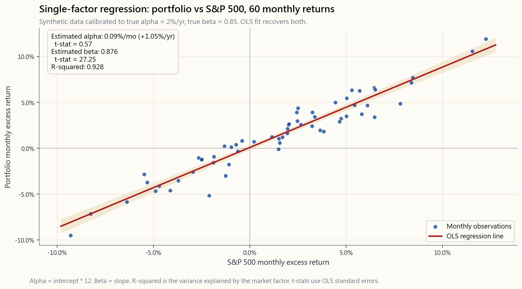
The chart in §2.1 shows what this looks like in practice on five years of monthly data calibrated to a portfolio with $\alpha = 2\%$ per year and $\beta = 0.85$. The dots scatter, the line slopes up, and the intercept reads about 17 basis points per month — exactly the 2%-annualised alpha we baked in. The cloud of dots above and below the line is $\varepsilon$: the part this single factor cannot explain, which is where multi-factor regressions go to work.

The Fama-French extension simply adds more right-hand-side terms:

$$R_p - R_f = \alpha + \beta_1 \cdot \text{MKT} + \beta_2 \cdot \text{SMB} + \beta_3 \cdot \text{HML} + \beta_4 \cdot \text{UMD} + \varepsilon.$$

Run this regression on a small-cap value fund and you will discover that its "alpha" from the one-factor model — say 4% per year — was actually a $\beta_2$ loading of 0.40 on size and a $\beta_3$ loading of 0.30 on value, multiplied by the 1963-2024 SMB and HML premia we catalogued in Week 23. Subtract those and the residual alpha is near zero, and not statistically distinguishable from it. Three percent of the four was factor compensation, not skill. That is the same finding S&P SPIVA prints every year; the regression is just the mathematical statement of why.

2.2 Residuals as the working definition of alpha

The intercept is alpha-on-paper; the residuals are alpha-in-process. A skilled manager generates not just a positive intercept but a residual series whose t-statistic survives the noise. If a fund has alpha of 0.20% per month with a residual standard deviation of 2% per month over 60 months, the t-stat is

$$t = \frac{0.20\%}{2\%/\sqrt{60}} = \frac{0.20\%}{0.258\%} \approx 0.78.$$

That is not statistically significant — there is no way to distinguish that intercept from zero with sixty data points and that much noise. You need either a longer window, a higher alpha, or a lower residual vol — typically all three — for the t-stat to clear the conventional 2.0 threshold. Alpha is rare, and the t-stat is the arithmetic of how rare. A 2% alpha at 5% residual vol needs roughly 25 years of monthly data before its t-stat trips 2.0. Twenty-five years. That is how long it takes to prove skill at that magnitude — not detect it, prove it. Most managers have not been managing money for twenty-five years.

2.3 Cross-sectional regression for stock picking

The CAPM regression is time-series: one fund, T monthly returns, one slope. The other family is cross-sectional: one date, N stocks, fit returns against current-snapshot characteristics.

$$r_{i,t+1} = \gamma_0 + \gamma_1 \cdot \text{B/M}_{i,t} + \gamma_2 \cdot \text{Size}_{i,t} + \gamma_3 \cdot \text{Mom}_{i,t} + u_{i,t+1}.$$

You run this for every month, collect the time series of $\gamma_1, \gamma_2, \gamma_3$ slopes, and average them. The average $\gamma_j$ is the realised premium per unit of factor exposure, and its t-stat tells you whether the factor pays. This is the Fama-MacBeth procedure (1973), and it is still the workhorse of academic factor research half a century later. Every "barra-style risk model" you have ever seen on a sell-side desk is some flavour of cross-sectional regression.

The retail use-case is signal building. You take a universe of 500 stocks, score each on (book-to-market, profitability, 12-month momentum), regress next-month returns against those scores, form the long-short portfolio implied by the slopes, and rebalance. That is the inside of every smart-beta ETF.

2.4 Time series: AR, MA, ARMA, and the random walk benchmark

For pricing series, the unconditional first question is: is this a random walk, or is there persistence? An AR(1) model

$$r_t = \phi \cdot r_{t-1} + \epsilon_t$$

estimates the autocorrelation $\phi$ at lag one. If $\phi > 0$, returns trend (this week's move predicts next week's). If $\phi < 0$, returns mean-revert. For US monthly equity returns the realised $\phi$ is about $+0.10$ — barely distinguishable from zero, which is why monthly stock returns are essentially impossible to forecast from their own history. For daily equity returns $\phi$ is mildly negative (microstructure mean-reversion); for cross-sectional relative returns at the 6 to 12-month horizon $\phi$ is mildly positive (Jegadeesh-Titman momentum, the cross-sectional momentum effect). Where $\phi$ is zero, no model that takes only past prices as input can win.

MA(q) and ARMA(p,q) models layer in moving-average residual terms to capture the news-arrival shock structure. In practice, for liquid equity returns, the best ARMA fits beat the zero-mean-random-walk benchmark by a few basis points of monthly RMSE — economically irrelevant after costs. For volatility series, on the other hand, AR-style models are wildly successful: volatility is highly persistent ($\phi \approx 0.95$ on daily VIX), which is why GARCH and HAR-RV models genuinely forecast tomorrow's volatility from today's. The volatility tail wags the return dog, and a lot of that asymmetry shows up here. You return dog — gets a lot of its leverage from this asymmetry. You cannot forecast next month's return; you absolutely can forecast next month's variance.

2.5 Rolling vs expanding windows, and the parameter-stability problem

Once you commit to fitting a model on history, the next choice is whether to use all of history (expanding window: at month $t$, fit on data from inception through $t-1$) or only the recent past (rolling window: at month $t$, fit on the last 60 months). Expanding windows have more data and therefore tighter estimates, if the underlying parameter is stable. Rolling windows adapt when the parameter changes, if the regime change is real and not noise.

There is no theoretically correct answer; there is only a parameter-stability test. For a CAPM beta on a megacap stock, expanding-window estimates from 1990-2024 give a roughly fixed beta — the parameter is stable and rolling adds noise. For the HML factor's market beta, on the other hand, expanding-window estimates are nonsense — the factor's beta on the market shifted sign in 2007. There the rolling window is mandatory. The practical default is a rolling 36-60 month window for monthly data, with a Chow break test for whether the parameter has shifted.

2.6 Train/validation/test, and the walk-forward defence

Every machine-learning pitch you will ever hear in finance involves the same vulnerability: the model was tuned on the same data its out-of-sample performance is reported against. The standard defense is a three-way split.

• Train (e.g. 1990-2010): fit model parameters.
• Validation (e.g. 2011-2017): tune hyperparameters — number of

features, regularisation strength, depth of tree, etc. The model is re-fit with each hyperparameter setting on train, scored on validation, and the best hyperparameter chosen.

• Test (e.g. 2018-2024): the model is evaluated exactly once

with its frozen hyperparameters. No re-tuning.

The brutal fact is that the test set, in an honest pipeline, is used once and then discarded. You cannot iterate on a strategy against the test set without it becoming a second validation set. Walk-forward validation generalises this: at every point in time $t$, the model is fit on data through $t-1$, used to predict $t$, and the next $t$ is appended to the training set. The realised out-of-sample performance is the only honest performance estimate.

The danger is the opposite of what most retail investors think. Overfitting does not look like a slightly-too-good in-sample result; it looks like a spectacularly good in-sample result that collapses to nothing — or worse, to negative — on the test set. The chart in §2.7 shows the canonical hump.

2.7 Overfitting, multiple testing, and the false-alpha mill

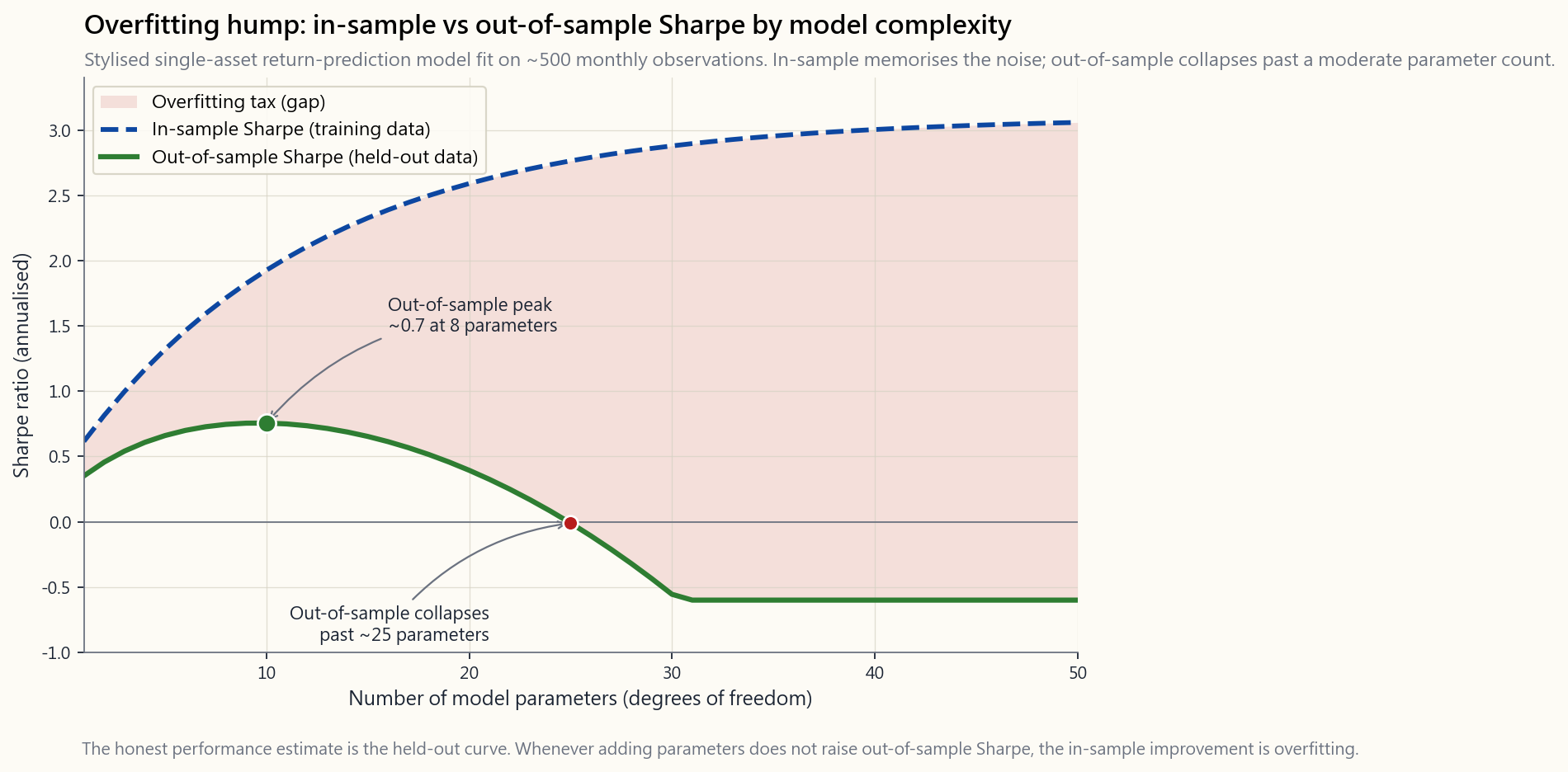
The classical curve has in-sample Sharpe rising monotonically with model complexity (more parameters, deeper trees, more features) — because with enough free parameters you can memorise the noise. Out-of-sample Sharpe rises briefly, peaks at some moderate complexity, and then collapses. The gap between the two curves is the overfitting tax. It is the single most reproducible phenomenon in empirical machine learning, and it is universal: it shows up in equity prediction, options pricing, credit scoring, and ad-click models alike.

The financial twist on top of this is multiple testing. Every researcher who tries a strategy and abandons it without publishing contributes to the survivorship of the strategies that happened to look good. If a hundred quants each try fifty signal variants on the same dataset, the combined family-wise error rate at $p < 0.05$ is essentially one. Marcos Lopez de Prado's Deflated Sharpe Ratio formalises this: the Sharpe at which a strategy must come in to beat the noise of having tried N alternatives is roughly $\sqrt{2 \log N}$ standard deviations of the null. Try a thousand strategies and the bar is roughly $\sqrt{2 \log 1000} \approx 3.7$ standard deviations of the unconditional Sharpe-noise — which on a 5-year backtest is a Sharpe of about 1.6 just to clear the bar of having looked. Most published anomalies do not clear it.

2.8 Why most ML alpha is feature engineering

Lopez de Prado's Advances in Financial Machine Learning (2018) makes the point in two slogans. "The model is the easy part." *"Most of the work is in labelling the target and engineering the features."* The reason is that financial data has a vanishingly low signal-to-noise ratio (about 0.05 R-squared per month for the best-fit linear model on equity returns), severe non-stationarity (the signal you found in 2010 may not work in 2020), and a labelling problem (was that price move a regime change, or microstructure noise?). The model — random forest, XGBoost, neural network — is largely a commoditised step. The differentiation sits in the features (which transformations of price/volume/order flow you fed in) and the labels (whether a 1% move counts as "+1" or you weighted by triple-barrier exits).

For the retail investor, the consequence is uncomfortable: the serious money in quant alpha is almost never made by training yet another XGBoost on yet another OHLCV dataset. It is made by sourcing or constructing features no one else has — alternative data, satellite imagery, credit-card panels, supply-chain text embeddings. The information lane of alpha is real but expensive. expensive. The "structural" lanes (liquidity, factor compression, vol-tail mispricing) remain the cheaper and more durable game for a single account.

---

3. Common Misconceptions

"R-squared 0.9 means the model is good." R-squared measures

variance explained, not predictive power. A regression of fund returns on the S&P with R-squared = 0.95 just means the fund is correlated with the market. It tells you nothing about whether the fund's alpha is real or whether you can forecast either series from anything.

"My backtest Sharpe is 2.5 in-sample, so the strategy works."

In-sample Sharpe is, on average, optimistically biased by roughly $\sqrt{N}$ standard deviations where N is the number of variants you tried. A 2.5 in-sample Sharpe routinely walks forward to 0.3.

"P-value below 0.05 means the result is real." A p-value below

0.05 means the probability of observing this result *given the null is true* is below 5%. With a thousand simultaneous tests, the expected number of false positives at p < 0.05 is fifty. Without a multiple-testing correction, "p<0.05" is barely an anchor.

"More data is always better." More data is better only if the

underlying data-generating process is stable. Adding 1990s data to your TIPS-breakeven model when TIPS did not exist before 1997 is not "more data," it is contamination.

"Out-of-sample Sharpe of 1.0 = great." Out-of-sample Sharpe of

1.0 net of transaction cost on a strategy whose features were chosen in 2010 and tested through 2024 is great. Out-of-sample Sharpe of 1.0 gross of cost on a six-month holdout that the researcher iterated against forty times is meaningless.

"Machine learning finds patterns humans miss." Machine

learning fits flexible functions to whatever you feed it. With N parameters, an unregularised model can fit any pattern in N-1 data points — including the noise. Whether the pattern it found is real is a question the model itself cannot answer.

"Cross-validation eliminates overfitting." K-fold cross

validation does not work for time series — it leaks future information into the training fold. The only valid CV for financial data is walk-forward with embargo (Lopez de Prado §7), and even then the test set is consumed once.

"Beta is constant." Beta is a regression slope on a finite

window. It is estimated with error and changes through time. Famously, the beta of value stocks against the market shifted from positive to roughly zero around 2007.

"My factor exposure regression has alpha. I have skill."

Statistically-significant alpha in a five-factor regression on a 60-month window is not, on its own, a skill demonstration. You need the t-stat, the residual diagnostics, and ideally a separate holdout. Twenty-five years of data, if not more.

"Quant models replaced traders." In aggregate, quant equity

market share has been about 30-40% of US dollar volume for the past decade. The remainder is humans, and a great deal of the quant share is execution, not signal generation. The interesting money is split.

---

4. Q&A Section

**Q1. If a regression gives my fund alpha = 1.5% per year and t-stat = 1.4, what should I conclude?** Nothing. T-stat 1.4 corresponds to a one-tailed p-value of about 8%, two-tailed about 16%. You cannot reject the null that the true alpha is zero. The estimate is consistent with skill and consistent with luck. You need more data, a higher alpha, or both before you can draw any conclusion.

Q2. How long do I need to evaluate a manager? Roughly 25 years for monthly data if the alpha is 2% per year and the residual vol is 5% per year — at which point the t-stat just clears 2.0. If the residual vol is higher (a typical hedge fund), multiply. The implication is uncomfortable: most "great" track records are not statistically distinguishable from luck.

**Q3. What R-squared should I expect on a single-factor CAPM regression of a US large-cap fund versus the S&P 500?** 0.85 to 0.95 is normal. An R-squared of 0.99 means the fund is a closet indexer (you should pay nothing). An R-squared of 0.50 means the fund is taking large factor or sector bets and you should run a multi-factor regression to see what they are.

Q4. Why is autocorrelation of monthly equity returns near zero? Because if it were materially positive, momentum strategies would arbitrage it away to zero, and if it were materially negative, mean-reversion strategies would do the same. The residual near-zero is the equilibrium. It survives at the cross-sectional level (relative momentum across stocks at 6-12-month horizons) where the arbitrageable shape is messier and slower.

Q5. What is "look-ahead bias" in practice? Using information you would not have had at the moment you traded. Common examples: backtesting a "buy when P/E < 15" rule using the P/E based on full-year reported earnings (which were only known months later), using GDP-revision data (revised down years after the fact) as if it were the print, or using reconstructed index constituents that exclude companies that went bankrupt mid-history. Survivorship bias is a special case.

**Q6. What is the difference between in-sample, validation, and out-of-sample?** In-sample: data the model was fit on. The fit is, mechanically, good. Validation: data used to choose hyperparameters. Independent of training but consumed in the tuning step. Out-of-sample / test: data the model has never seen. A correctly-built pipeline runs the test set exactly once, after the entire model — including hyperparameters — is frozen.

Q7. How many parameters can I use before overfitting? The rule of thumb on linear models is 10-20 observations per parameter as a minimum. For non-linear models with many degrees of freedom (random forests, neural nets) the answer depends on regularisation; the empirical defense is walk-forward Sharpe — if adding parameters does not improve walk-forward Sharpe, the in-sample improvement is overfitting.

Q8. Should I use ML or linear regression for stock prediction? Linear regression first, always. If a linear model on well-engineered features cannot find a signal, an ML model on the same features will not find one either; it will just overfit faster and feel like skill. ML earns its keep when the underlying relationship is actually non-linear, and you have enough data to estimate the non-linearity, and you have a feature set that the linear model cannot exploit. That is a small intersection.

Q9. What is "data mining" and what is wrong with it? Data mining is searching a large space of strategies for what fits past data. Mathematically it is fine; what is wrong is reporting the best one as if it had been the only one tried. Without a multiple-testing correction, the reported Sharpe is biased upward by the size of the search. Lopez de Prado's deflated Sharpe is the standard fix.

Q10. Why is feature engineering more important than the model? Because financial data is low signal-to-noise and the marginal return on model complexity is sharply diminishing. Two competing shops with the same features and different ML models tend to converge to similar Sharpe ratios; two shops with the same ML model but materially different feature sets diverge sharply. The features are where the information sits.

Q11. Can I run these regressions myself? Yes. Python's statsmodels or scikit-learn, or R's lm(), run a five-factor regression in two lines. Kenneth French's data library publishes the FF5 + UMD monthly factor returns for free, 1963 to present. Subscript the time series, regress, read off alpha and t-stat. The week's interactive lab does the basic single-factor version inline.

Q12. What is the single most important habit? Always reserve a holdout. Always. Whatever fraction of your data you can spare — 20%, 30%, the last three years — reserve it before you do anything else, and do not look at it. When the strategy is final, exactly once, score it on the holdout. The number you get is the only honest number you will have. "Alpha is rare" stops being a slogan and becomes intuitive the first time you watch a strategy's in-sample Sharpe of 2.5 walk forward to 0.4.