Week 47: Tail Risk — Universa, Put Protection, and CTAs as Long-Vol Diversifiers

---

1. Why This Is Important

A black swan, in the way the textbook teaches it, is a 5σ event: five standard deviations below the mean of a normal distribution. Under the bell curve, that occurs once every 14,000 years. The S&P 500 had three of them between 1987 and 2020 alone.

Markets do not deal in normal distributions. The 1987 single-day −22.6% close was, on the parametric assumption financial economists were teaching that morning, a once-in-10⁵⁰-year event — many orders of magnitude longer than the age of the universe. It happened on a Monday. The −12.0% single-day move on March 16, 2020, was a "5.6σ" print. The Volmageddon −115% one-day VIX-product implosion of February 5, 2018 was — under the model that priced those products — a once-in-the-life-of-the-sun event. That makes four lifetimes of the universe in three decades, all of which the same investors lived through.

Tail risk is the part of the distribution the textbook erases. This lesson is about the small slice of the portfolio that is designed to be paid when the textbook erasure shows up.

You need to understand tail-risk hedging for four reasons:

The arithmetic of drawdowns is non-linear. Down 50%

requires up 100% to get back. Down 75% needs up 300%. A portfolio that sidesteps the worst 5% of months over a long horizon ends up, mechanically, at a higher terminal wealth than one that earns a slightly higher mean return without the protection. Tail-risk hedging is a way to manufacture that arithmetic — buy the right to sell at a price that only matters when prices have collapsed.

Diversification breaks exactly when you needed it. In

normal regimes, stock-bond, US-EM, and value-growth correlations are moderate. In a crisis they spike toward +1. The 60/40 you read about in Week 4 lost roughly 22% in 2022 because the diversifier ran out of negative correlation. Tail hedges are the only negatively-convex sleeve that gets more negatively correlated the worse the loss — exactly the property that fails in everything else.

**Long-vol carry is small but bounded; tail-vol payoff is huge

but rare.** This is the barbell at the portfolio level. Spend a known small drag — 50 to 150 basis points per year — for a very large unknown payoff in a crash. The mirror of selling premium (Weeks 26–30): there, you collect a known small premium for a known small risk and one big tail. Tail hedging is the buyer side of that same trade. The underlying claim — the volatility tail wags the dog — is that the few crash days dominate the return distribution, so paying to be on the right side of those days is rational even if the carry hurts.

**CTAs and managed futures are the systematic, naturally-long-

vol alternative.** Trend-followers do not buy puts. They go short on the way down by following the trend signal. In 2008 the SocGen CTA Index returned roughly +14% while the S&P 500 lost 38% and a 60/40 lost 22%. The mechanism is different — a long straddle synthesised from many trends rather than a literal option — but the convex-payoff shape in a crash is similar. That is why allocators pair CTAs with stocks the same way they would pair OTM puts with stocks: as a long-vol diversifier that earns very little in calm years and rescues the portfolio when correlations break.

---

2. What You Need to Know

2.1 What "Tail" Actually Means in Markets

The 1928–2024 daily S&P return distribution is not normal. It is fat-tailed — leptokurtic in the technical language, kurtosis around 20+ vs. 3 for the bell curve. The tail count is not abstract. Using daily data:

• 3σ days (about ±3% on the day): Normal distribution predicts

about one every 1.5 years. Observed: roughly 5–8 per year on average, and clustered around crises.

• 5σ days: Normal predicts one every 14,000 years. Observed:

about every 3–5 years.

• 10σ-equivalent days like 1987 or March 16, 2020: Normal

predicts essentially never. Observed: a handful per investing lifetime.

Because the empirical tail is much heavier than the parametric tail, two things follow. First, any model that uses normal distributions for risk — VaR, Sharpe ratios, CAPM-based pricing — systematically underprices crash risk. Second, the actual expected dollar contribution of those tail days to the long-run portfolio is not small. A handful of −10% days dominate decades of average returns. The tail wags the dog.

2.2 The Cost-of-Insurance Tradeoff

The classic tail hedge is an out-of-the-money put on the index. On April 2026, with SPY trading near $520, the rough quotes for a 90-day put are:

Strike	% OTM	Premium ($)	Premium / Notional	Payout if SPY = $364 (−30%)
$500	4%	$9.30	1.79%	$13,600 / contract
$470	10%	$4.50	0.96%	$10,600 / contract
$440	15%	$2.10	0.48%	$7,600 / contract
$400	23%	$0.65	0.16%	$3,600 / contract
$360	31%	$0.20	0.06%	$0 / contract

(Black–Scholes at σ = 19%, r = 4.3%, q = 1.3%.)

The 15% OTM put costs about 0.48% of notional for a 90-day window — call it ~2% of notional per year if rolled quarterly. In a crash to −30%, $1 of premium turns into roughly $36 of payout (a ~36× MOIC on the hedge sleeve), which on a 50bps allocation translates to about +18% on the whole portfolio.

But that 2%/year drag in normal years is what kills most retail attempts at this. Spend 2% protecting against an event that happens once a decade and you are −20% cumulatively versus the unhedged stock by the time the event arrives. That is why Universa's framing is different: spend less (50–150bps/yr) on deeper-OTM strikes that are cheap in normal times but explode in convexity in a crash.

2.3 The Universa-Style Architecture

Universa Investments — Mark Spitznagel's firm, with Nassim Taleb as advisor — popularised what they call the *capital-efficient tail hedge*. The architecture, as publicly described:

• Hedge size: 0.5% to 2% of NAV per year, depending on regime.
• Strikes: deep OTM (typically 25–35% OTM on the index).
• Tenor: rolling, weighted toward the 1- to 3-month part of

the surface where vol-of-vol is highest.

• Behaviour in normal regimes: cost is a slow drag — most

options expire worthless.

• Behaviour in a crash: the gamma profile of deep-OTM puts

goes parabolic. Universa publicly disclosed in March 2020 a +4,144% return on the hedge sleeve for that month, which the firm and Taleb have framed as turning a stock-portfolio crash from a −30% drawdown into an ~+0.4% total-portfolio gain when paired in a 3.3 / 96.7 ratio of hedge sleeve to risk assets.

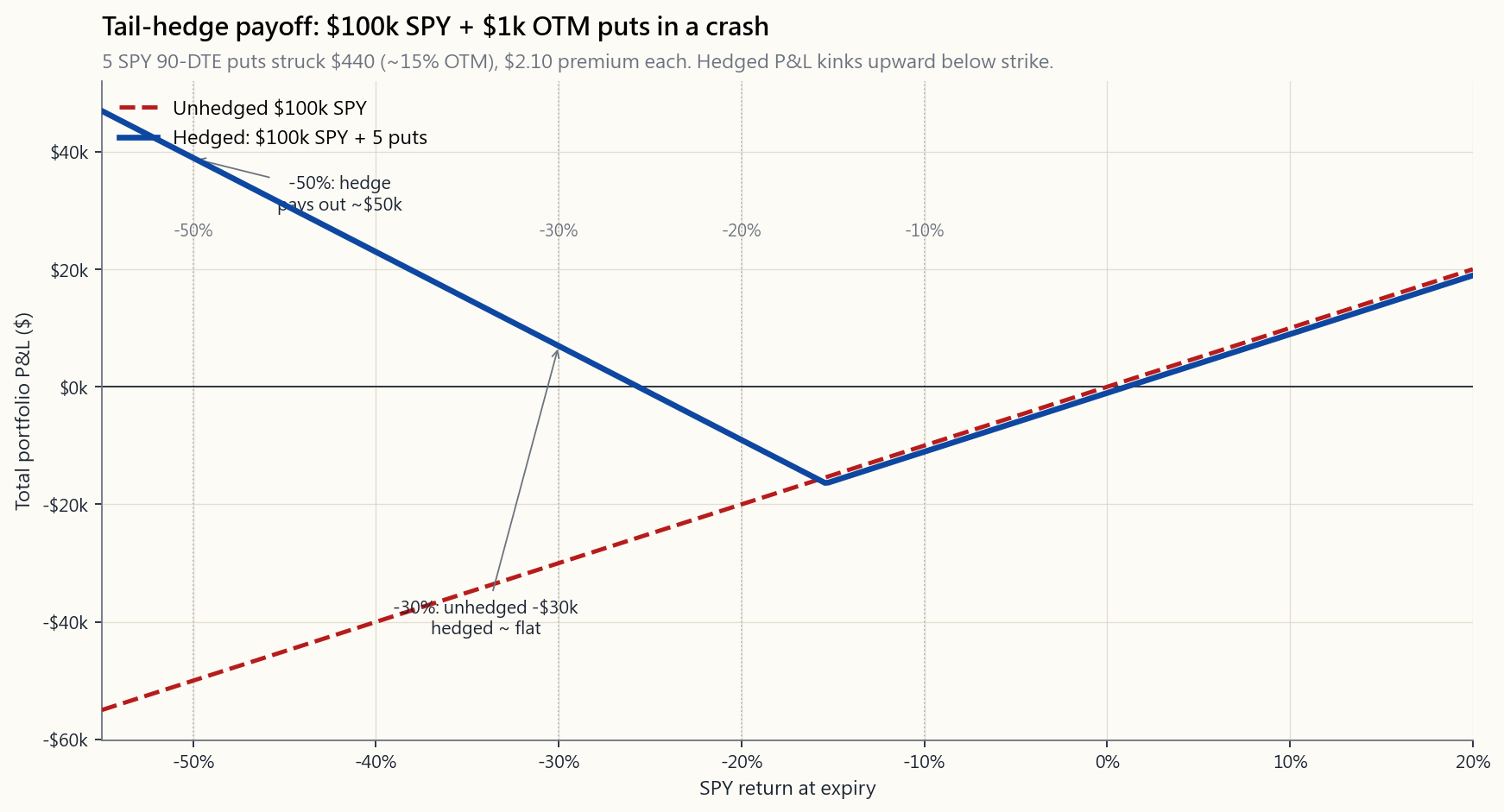
The chart below shows the geometry on a hypothetical $100,000 S&P 500 position with a $1,000 quarterly tail-hedge budget. In a −30% scenario, the unhedged $100k loses $30k; the $1k put-hedge sleeve, sized at 5–10% OTM strikes rolling at quarterly horizons, returns roughly 25× to 50× — turning a −$30k drawdown into a small positive or near-zero combined P&L.

The tradeoff to internalise: every quarter the market does not crash, that $1,000 evaporates. Annualised, you are giving up 4% on the hedge sleeve, or roughly 1% of the total portfolio. That is the price of carrying the convex insurance. The empirical question is whether that 1%/year drag is recouped — and then some — in the crash that historically arrives every 7–10 years.

2.4 CTAs and Managed Futures as Long-Vol Without the Premium Bleed

A second, structurally different way to be long the tail is to be long trend. Managed-futures programmes — sometimes called CTAs, for Commodity Trading Advisors — run systematic trend-following across roughly 50 to 200 liquid futures markets: equity indices, rates, currencies, commodities, and volatility itself. The signal is some flavour of "buy what is going up, sell what is going down, let the position size scale with realised vol."

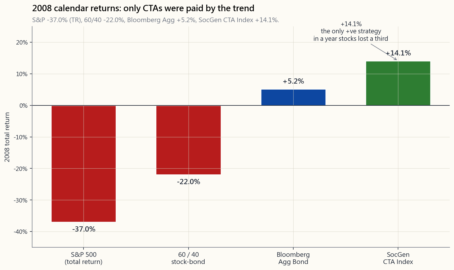
A trend-follower's payoff diagram across an uninterrupted six-month down-move looks structurally like a long straddle on the underlying — small chop in calm regimes (because trends whipsaw), large positive payoff during sustained directional moves. That is exactly the regime a crash creates. In 2008:

Strategy	2008 calendar return
S&P 500 (total return)	−37.0%
60 / 40 stock-bond	−22.0%
Bloomberg Aggregate Bond	+5.2%
SocGen CTA Index (managed futures)	+14.1%
Universa-style tail hedge (modelled)	+50% to +100%+

The mechanism for CTAs is not that they own crash insurance. It is that the trend up to the crash had already moved them short equities, long bonds, and long the dollar by the time the crash arrived. They are paid by the persistence of the move, not by the shape of the implied vol surface. This makes them a different kind of long-vol exposure — long realised vol, not long implied vol — with the crucial property that the carry cost is much lower in a normal year (often near zero or modestly positive) than the direct put-buying programme.

The catch: CTAs underperform during crisis-then-snap-back regimes, because the trend signal whipsaws. Q4 2018, March 2020, and the 2022–23 sequence are textbook examples where CTAs were short stocks into the bottom and then chopped on the way back up. Direct put hedging delivers cleanly on a single down move and is paid out immediately. CTAs need the move to persist. Both are long-vol exposures, but the failure modes are different.

2.5 The Barbell at the Portfolio Level

This is the barbell at the portfolio level. Most of the portfolio sits in the slow-compounding base — index equities, T-bills, gold, the boring part. A small sleeve, 1% to 5%, is the convex tail hedge: deep- OTM puts, VIX calls, or a CTA programme. The expected return on the small sleeve in any single year is negative (for puts) or roughly zero (for CTAs in chop). The expected return *conditional on a crash* is enormous.

The barbell logic:

• Bounded downside on the hedge sleeve. The most you can lose

on the puts is the premium. There is no margin call, no liquidity event, no forced unwind. The hedge cannot blow up in a way that hurts the rest of the portfolio.

• Unbounded upside on the hedge sleeve. A 30× or 50× hedge

payoff is not unusual in a crash. The 2020 prints of 1000%+ for 1-week deep-OTM SPY puts are documented.

• Net portfolio exposure becomes positively skewed. You have

given up a small, known expected return for a much larger expected return in the left tail. This is the same trade as Week 14's barbell — small known bad outcome, large unknown good outcome — applied to the insurance leg of the portfolio rather than the upside leg.

2.6 Sizing the Hedge — Three Practical Rules

Cap the carry at 1% of total NAV per year. That is roughly

the upper bound of what backtests support being recouped on long-horizon crashes. Going higher than this turns the hedge from insurance into a directional bearish bet.

Roll quarterly, not annually. Monthly is too expensive

(theta crushes the sleeve), annually leaves too much gamma on the table during a fast move. The 60–90 DTE window with a quarterly roll is the published Universa cadence.

**Strike selection: pick the cheapest strike where premium /

notional ≤ 0.5%.** This is typically 15–25% OTM at moderate IV, and 5–15% OTM in a high-VIX regime. Cheaper strikes pay more in convexity; richer strikes burn the carry budget too fast.

For most retail investors the practical implementation is: hold SPY (or VTI), set aside a 1% sleeve, buy 90-day SPY puts at the strike where premium / notional ≈ 0.4%, and roll on the same calendar each quarter. Total carry: ~1.6%/yr at IV ≈ 18%, less when IV is low. Index puts taxed under the 60/40 long/short rule (Section 1256 contracts) get an edge worth ~200bps after-tax for most investors.

2.7 What This Is Not

• Not market timing. The hedge is on continuously, not bought

before perceived crashes. The signal-to-noise ratio for "crash prediction" is too low to be tradable.

• Not a substitute for asset allocation. A barbell with no

base is just a deep-OTM put portfolio. The base — index equities, T-bills, gold — is what compounds. The hedge protects the compounder.

• Not free. Annual carry of 0.5% to 2% is real money. The

hedge needs to be sized so the carry is tolerable in a 7–10 year no-crash window. The interactive lab below lets you stress-test exactly that tradeoff.

The interactive week47_tail_lab.html lets you set the budget, the strike, the DTE, and the crash scenario, and reads off the hedge cost, hedge payoff, drag in normal years, and unhedged-vs-hedged drawdown side by side.

---

3. Common Misconceptions

"Black swan = 5σ event." No — a black swan is, by Taleb's

own definition, an unmodelled event. The 5σ language is the normal-distribution approximation of how rare textbooks thought it was. Real markets generate "5σ" events on a schedule that has nothing to do with the bell curve.

"Tail hedging is the same as buying puts." Buying ATM puts

is portfolio insurance — expensive (~6–8%/yr drag), and most of what you pay for is implied vol you don't actually need. Tail hedging is the deep-OTM convex slice. Different product, different cost structure, different payoff geometry.

"If puts always lose money, why buy them?" Because the one

year they pay off, they pay 30–100×. The geometric mean of a distribution with one big positive realisation and many small negative realisations is not the arithmetic mean of the slice — it is the compounded portfolio path. Adding a negatively- correlated convex slice can raise the geometric mean even if the slice's own arithmetic mean is negative.

"CTAs are just a hedge fund strategy with high fees." CTAs

charge fees, but the long-vol convex payoff is the structural feature, not the fee structure. The cleaner retail proxy is now liquid: KMLM, DBMF, CTA, RPAR-like products in the US. Annualised cost is closer to ETF rates (50–100bps) than hedge- fund 2-and-20.

"VIX calls are the right tail hedge." VIX calls are

leveraged on implied vol, which mean-reverts hard after a crash. Many of the famous VIX-call payoffs are gone within a week, before retail can monetise them. SPY/SPX puts settle on the underlying, not on a mean-reverting volatility index, and so the payoff is captured cleanly.

"60/40 hedges itself." It did from 1990 to 2021, when

stock-bond correlation was negative. In 2022 both legs fell ~18% together. A 60/40 with no explicit tail hedge has no protection in regimes where rates and equities sell off together — exactly the inflation-driven left-tail regime.

"Tail hedges underperform forever, then pay off once."

Closer to: tail hedges underperform during long quiet periods and pay off in the 5–10% of months that matter. The cumulative contribution of those months is what you are buying. Compounding is path-dependent.

"Universa just got lucky in March 2020." Possible. But

the same firm reported strong tail-payoff numbers in 2008, 2011, 2015, and 2018 — a pattern more consistent with a structural strategy than with single-event luck. The strategy mechanism — deep-OTM put rolling — is publicly replicable and the math is well-understood.

"I can just sell when the market falls." The historical

record on retail timing is brutal (Week 11). A hedge sleeve is on automatically — no decision required at the moment of panic, which is when investors are least able to act rationally.

"Tail hedges are only for the wealthy." A 1% sleeve on a

$100k portfolio is $1,000/yr. SPY options are penny-priced at deep-OTM strikes. The minimum-viable implementation is one $440-strike SPY put at $2 ≈ $200, four times a year ≈ $800/yr. Within reach of any retail brokerage account with options approval.

---

4. Q&A Section

**Q1. What's the simplest tail-hedge implementation a retail investor can run?** A. Hold SPY (or VTI, but the SPY/SPX option chain is more liquid). Each quarter buy one or two 90-day SPY puts struck at roughly 15% OTM, sized so the total annual premium spend is 1% of the portfolio. Roll the puts on the same calendar each quarter — do not skip a quarter just because the market is calm.

Q2. What about VIX calls instead of SPY puts? A. VIX calls have a more violent gamma profile during a crash spike but mean-revert hard within days. The window to monetise is short, and most retail traders do not have the discipline to sell into a VIX print of 60+. SPY puts settle on the underlying, not on a mean-reverting index, and are easier to manage. Some managers blend the two — VIX calls for the spike, SPY puts for the sustained drawdown.

**Q3. Should the hedge be on the whole portfolio or just the equity sleeve?** A. Just the part that has equity-like beta. If you are 60% SPY, 20% bonds, 10% gold, 10% T-bills, the hedge is sized on the 60% SPY position (and on whatever fraction of the 20% bonds is long-duration, which has its own drawdown risk).

Q4. How does the cost change with the VIX level? A. Linearly with implied vol, roughly. At VIX = 12 the deep-OTM strikes are very cheap (premium / notional ~0.2%); at VIX = 30 the same strikes cost 2–3× as much. Universa-style programmes reduce hedge spending in high-IV regimes and increase it in low-IV regimes. Cheap insurance is the right time to buy insurance.

Q5. Why do CTAs lose money in chop but make money in trends? A. The trend signal needs price persistence in one direction. A market that rallies 10%, falls 10%, rallies 10% over three months generates whipsaw losses — the strategy buys the rip and gets stopped out, sells the dip and gets stopped out. A market that falls 30% over three months is a clean trend the algorithm rides short for the entire move. 2008 was a clean trend; Q4 2018 and March 2020 were closer to chop with snap-back.

Q6. Can I do both — puts and CTAs? A. Yes, and it is a common institutional setup. A 5% allocation to a CTA ETF (KMLM, DBMF, or similar) and a 1% put-hedge sleeve gives you long-realised-vol and long-implied-vol exposure. The two profiles are complementary: CTAs cover the slow-developing trend, puts cover the gap-down event.

**Q7. Is tail hedging a positive expected-return strategy in isolation?** A. The hedge sleeve itself has negative arithmetic expected return in normal regimes — that is the price of insurance. The portfolio-level expected geometric return can rise, however, because the convex payoff in left-tail months changes the compounding path of the whole book. The empirical record on isolated tail-hedge programmes shows roughly flat to mildly negative absolute returns across full cycles, but materially positive contribution to the host portfolio's compounding.

Q8. What is the worst-case for a tail-hedge sleeve? A. A long, slow grinding bull market with no volatility events. 2017 is the canonical example — the S&P returned +21.8% with realised vol below 7%. A 1% put-hedge sleeve was a near-total loss for that calendar year, contributing roughly −1% to total portfolio return. The bet is that the year you give up 1% is the year stocks are up 22%, so net exposure is fine. The bet fails if you have a decade of 2017s in a row, which has not historically happened but is theoretically possible.

Q9. How does this interact with leverage? A. Tail hedges enable leverage. A leveraged long-equity book without crash insurance can be liquidated by a single down move. With deep-OTM puts in place, the maximum drawdown of the hedged levered book is bounded — roughly the strike distance plus the hedge cost. This is the published architecture behind risk-parity- with-tail-hedge funds and some pension allocations.

Q10. Is now a good time to buy tail hedges? A. The answer is always yes, on schedule. Buying tail insurance in response to a perceived crash signal turns the strategy from a hedge into a directional bet, and the directional bet has terrible odds. The Universa argument is that you should be buying more protection when VIX is low and protection is cheap, not less. As of April 2026, VIX is around 14, which historically has been a favourable buying environment for deep-OTM SPY put protection.

Q11. Does this work outside US equities? A. The cleanest deep-OTM option market is SPX/SPY. EFA/IWM/IEFA have viable but thinner chains. EM puts are too illiquid for a systematic programme. Sticking to a US-listed investable universe, the practical retail implementation is a US-equity-base portfolio with a US-equity-index put hedge.

**Q12. What is the relationship between this and Week 40 (VIX) and Week 42 (VaR)?** A. Week 40 explained why VIX is a forward-looking measure of implied vol — the input that prices these puts. Week 42 explained why VaR systematically underestimates tail risk — the empirical problem this lesson solves. This week is the response to those two: the practical structure that takes the VaR underestimation seriously and uses VIX-priced options to do something about it.