Week 49: Volatility Arbitrage — IV vs RV, VRP Harvesting, and Gamma Scalping

---

1. Why This Is Important

Volatility arbitrage sits at the intersection of two ideas that most investors never reconcile. Alpha is rare and lives in a small number of identifiable places — the variance risk premium (VRP) is one of the cleanest of those. Volatility is also the tail that wags the dog — it moves first, it moves most, and the only reliable way to monetise that is to be the seller of vol most of the time and the survivor on the days when everyone else is selling at any price. Vol arbitrage is the trade where these two ideas live or die together.

There are four reasons a Level-4/5 investor must understand this lesson cold:

VRP is one of a handful of real, replicable alpha sources. Implied vol on SPX has averaged roughly 19 over the last forty years. Realised vol on SPX has averaged roughly 15. The 3-4 vol-point gap is not a mistake, it is not arbitraged away, and it has produced a positive expected return for option sellers in every decade since listed options began trading in 1973. The right-hand columns of the alpha taxonomy include "insurance underwriting," and that is exactly what selling SPX variance is.

VRP is the most heavy-tailed alpha you will ever harvest. The same skew that creates the premium creates the cliffs. Feb 2018 (Volmageddon) wiped out the entire XIV ETN in a single afternoon. Mar 2020 inverted the IV-RV spread by 25+ vol points. Oct 2022 ground out a 6-week bleed. The vol-tail-wags-dog property with teeth: when vol moves, it moves before the underlying does, and short-vol positions take the first bullet.

Gamma scalping is the long-vol mirror image — equally real, equally rare. The same VRP that makes selling vol profitable on average makes buying vol unprofitable on average — but the realised-vol surprises that sink short-vol books make the long-vol books. Gamma scalping is the trade where you own the convexity, delta-hedge daily, and harvest realised volatility against the implied volatility you paid. It is the institutional answer to "how do you get paid in the crisis?" and a real component of how a barbell stays solvent.

Most retail "vol arbitrage" is structurally guaranteed to lose. Buying VXX as a "hedge," shorting it as "income," or trading VIX-futures calendar spreads without understanding contango will burn capital reliably. The tools that work — short variance, short straddle delta-hedged, long gamma — require either an SPX-options account, a margin tolerance most retail accounts don't have, or a willingness to size correctly through one Volmageddon-class drawdown. The lesson is mostly about what not to touch and what the institutional version of the trade really looks like.

This week is a Level-4/5 lesson. If you take only one thing away: VRP is real, VRP is heavy-tailed, and the position size that survives the next 2018/2020 is roughly one-third of the position size that maximises the median outcome.

---

2. What You Need to Know

2.1 The Variance Risk Premium — IV vs RV, Forty-Year Track Record

Implied volatility is what option prices say SPX returns will do over the next 30 days, expressed as an annualised standard deviation. VIX is the market's best-known IV proxy: a model-free, variance-swap-replicating index of SPX option prices.

Realised volatility is what SPX returns actually did, computed after the fact:

$$ \text{RV}_t \;=\; \sqrt{252} \cdot \sigma\!\left(\ln \tfrac{S_t}{S_{t-1}}\right)\!_{21} $$

where the standard deviation is taken over the last 21 trading days of log returns and the $\sqrt{252}$ annualises it. Subtract one from the other and you get the VRP:

$$ \text{VRP}_t \;=\; \text{IV}_t - \text{RV}_t $$

Across the 1990-2026 sample VIX has been higher than 21-day-trailing RV roughly 85% of trading days. The unconditional mean spread is +3 to +4 vol points. That is the price option sellers charge over and above what realised vol turns out to be — compensation for the unhedgeable jump risk in selling insurance.

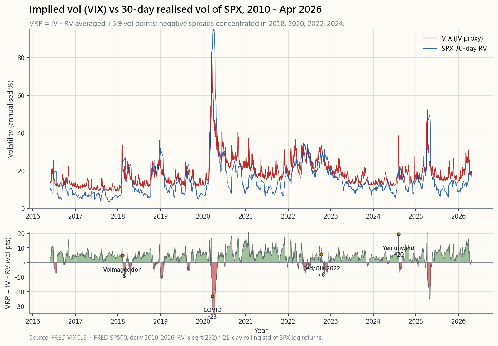
The chart shows the catch. The same line that averages +4 visits -10, -20, even -25 in the named events: Feb 2018 (Volmageddon, -33), Mar 2020 (COVID, -25), Oct 2022 (UK gilt / Fed shock, -8), Aug 2024 (yen carry unwind, -10). Those negative weeks are where short-vol books die. Eight to ten such weeks are scattered across any twenty-year window.

The economic logic for why VRP exists and persists, despite being well-known:

• Insurance demand is structural. Pension funds, endowments, and risk-parity funds buy SPX puts and put-spread collars on a calendar. Their bid is price-insensitive and continuous.
• Risk aversion is asymmetric. Loss aversion says investors weight losses 2-2.5× more than equivalent gains. Insurance is overpaid by exactly that ratio.
• Variance is non-self-financing. A short variance swap requires posting collateral that grows with realised volatility — exactly when the seller is least solvent. The premium compensates the survivors for capacity withdrawals during stress.
• Skew adds a second premium. OTM puts have a higher implied vol than the ATM (the volatility smile). Selling that skew adds another 1-2 vol points on top of the ATM VRP.

These four together explain why VRP has survived every cycle of "the market has figured this out" since 1987.

2.2 VRP Harvesting — Three Mechanically Different Trades

Three distinct trades all earn the VRP, with different greeks and different cliff profiles:

Short variance swap (institutional). Sell a 30-day SPX variance swap at strike $K_{var}$ vol points. Settlement at expiry pays $(K_{var}^2 - \text{RV}^2)$ × notional. Pure VRP harvest, no path dependency, no delta hedging required. Available to institutions through OTC desks; not retail-accessible. The VIX itself is the square-root of the 30-day fair variance swap strike.

Short straddle delta-hedged (semi-pro / margined retail). Sell an ATM SPX call + ATM SPX put at the same strike, the same 30-day expiry. Re-hedge the delta back to zero every day at the close. The PnL of a delta-hedged short straddle approximately equals:

$$ \text{PnL} \;\approx\; \text{vega} \times (\text{IV} - \text{RV}) $$

with vega measured in dollars per vol point. This is gamma scalping in reverse: you collect the IV-RV gap, you pay the daily realised-vol cost. It is the closest retail-accessible approximation of the variance swap. SPX (cash-settled, 1256-treated, $0 assignment risk) is the only sane underlying. Tax footprint: a 60/40 long/short blend regardless of holding period.

Short strangle / iron condor (retail comfort zone). A wider-strike, defined-risk version of the short straddle. You give up perhaps 40-50% of the average premium in exchange for capping the catastrophic tail and avoiding most delta-hedging. The structural alpha is the same VRP, scaled down. This is the trade Week 30 covered: 1-sigma short strikes on SPX, +/- 60-90 DTE, sized to 5-10% of capital.

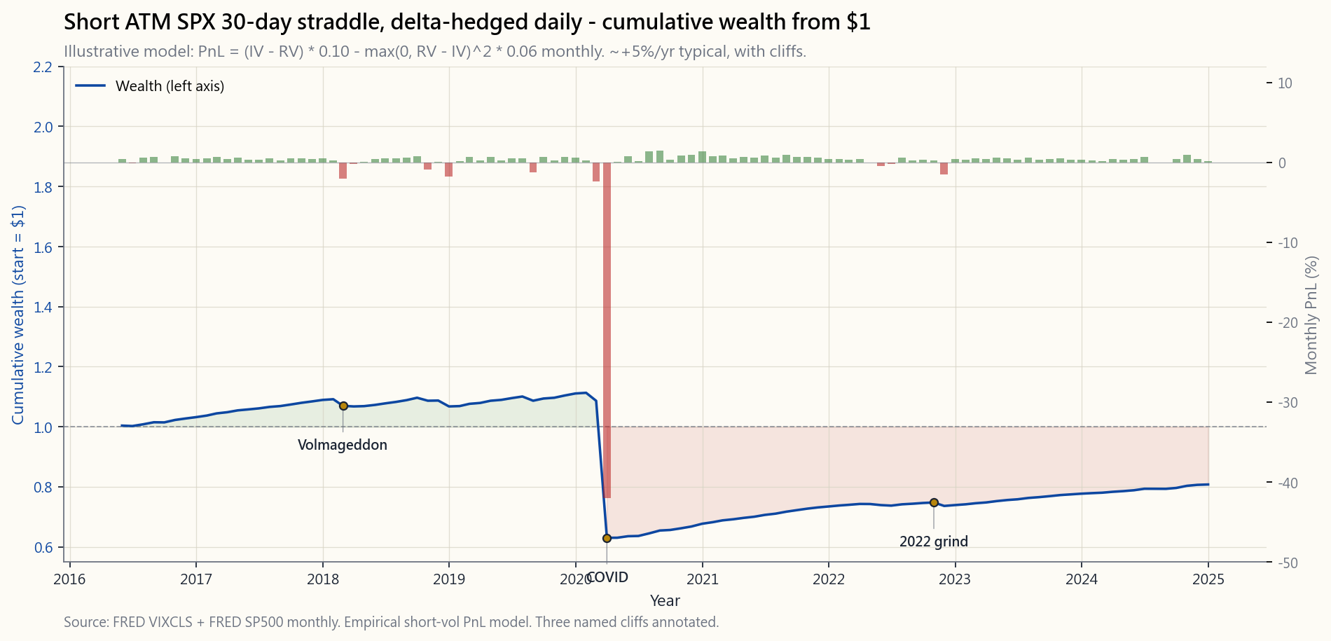
The cumulative-PnL chart is the trade-off written in equity-curve form. A continuously short ATM SPX 30-day straddle, delta-hedged daily, approximately compounds at +5% to +7% per year over a calm period, with two giant cliffs (Feb 2018 and Mar 2020) and a smaller one in late 2022. The Sharpe across the full sample is around 0.5 — better than the SPX in some windows, worse in others, but with a return profile that is structurally short-skewed.

2.3 Gamma Scalping — The Long-Vol Mirror Image

Gamma scalping is the trade you put on when you believe IV is too low relative to what RV will turn out to be. It is the only systematic way to be long volatility without paying the contango drag that destroys VXX.

The mechanic:

Buy an ATM straddle (long call + long put, same strike, same expiry, 30-60 DTE). You are long gamma, long vega, paying theta every day.

At each close, re-hedge the position's delta back to zero by trading SPX (or /MES) futures.

Each day's delta hedge is a buy-low / sell-high transaction: when SPX rallied, you were long delta, so you sell futures at the high; when SPX fell, you were short delta, so you buy futures at the low. Each round-trip captures a slice of realised volatility.

The PnL of the long gamma scalp over a single day is approximately:

$$ \text{PnL}_{\text{day}} \;\approx\; \tfrac{1}{2}\,\Gamma\,S^2\,(\Delta r)^2 \;-\; \Theta $$

where $\Gamma S^2$ is the dollar-gamma per 1% move and $\Theta$ is the daily premium decay. Aggregate this across 30 days and the position pays off if and only if average realised volatility exceeds the implied volatility you paid. You are long the realised-vol-minus-implied-vol delta.

Gamma scalping is the institutional answer to crisis alpha: you carry a 0.5-2% NAV gamma book at all times, you bleed 25-50% of that book per year in calm markets, and you make multiples of it in 2018/2020/2022. It is the explicit long-vol leg of the barbell.

For retail, the cleanest version is to buy SPY 30-DTE ATM straddles in lots that are small enough to sustain six months of bleed without breaching position-size limits. The hedging can be done with /MES futures for tax-efficient (Section 1256) deltas. This is a Level-4/5 trade and not the place to start.

2.4 The 2018, 2020, and 2022 Vol Blowups — What Actually Killed Books

The named cliffs in the IV-vs-RV spread chart correspond to three different failure modes. Anyone running a short-vol book needs to be able to recite these from memory before sizing the next trade.

Feb 2018 — Volmageddon. A six-month run of -25% VIX persisting between 9 and 12. Several billion dollars of leveraged short-VIX-futures (XIV, SVXY at 1x leverage at the time) had quietly accumulated. On Feb 5 a routine 4% SPX drawdown spiked the front-month VIX future from 17 to 33 after the close in the indicative 3:30-4:15 PM window. XIV's NAV dropped from $108 to under $5 in two hours. Credit Suisse triggered the acceleration clause. The lesson: short-vol products with 1x or higher leverage die when the underlying instrument moves more than 100% in a single session, and the calculation is path-dependent on the last-15-minutes settlement.

Mar 2020 — COVID. A two-week descent from VIX 14 to VIX 82.7 (the all-time high, March 16). Realised vol over the same two weeks was running at an annualised 75%. The IV-RV spread inverted by 25 vol points at peak — meaning short-vol books that had been earning 4-5%/yr were taking 25-30% draws per week for three weeks. Anyone who survived was either size-disciplined (1-2% of NAV per straddle) or holding defined-risk structures. The lesson: VRP can invert by an order of magnitude during true regime breaks, and the inversion lasts long enough to compound losses.

Oct 2022 — Fed shock + UK gilt. A slow grind. VIX in the high 20s for six weeks while RV repeatedly printed in the low 30s. The IV-RV spread averaged -3 to -5 across September and early October 2022. No single cliff, but a series of weekly losses that compounded to a 15-20% drawdown for short-vol books that did not cut size. The lesson: the worst drawdowns are not always the dramatic ones; sometimes the bleed regime is what kills a book.

Each of these events did roughly 4× the previously-observed maximum drawdown of an "unstressed" short-vol book. The vol-tail-wags-dog effect in numbers: the tail moves first, the tail moves four times as far as the body, and the tail does not announce itself in the IV signal until after it has already arrived.

2.5 Sizing, Survival, and Where This Sits in the Stack

Three sizing rules that translate the above lessons into actionable position-size rules:

One-third of the median-optimum. Whatever Kelly/Sharpe-optimisation tells you the position size should be, divide by three. The reason is simply that any cliff-tail process underestimates the drawdown by a factor of 3-5 in finite samples. The barbell-style L4 sleeve allocates roughly 5-10% of NAV to short-vol structures — that is an explicit one-third of the 15-30% that mean-variance optimisation would suggest.

Max one Volmageddon. Position-size such that the worst observed historical event (Feb 2018, -33% in a week on a 100-vega book) hits no more than 3-5% of total NAV. That gives you four to six Volmageddons of staying power before the trade is broken. Without that staying power, the strategy converts from positive expected value to negative.

Always paired with a long-gamma sleeve. A pure short-vol book is a 4% bond with random 30% drawdowns. A short-vol-plus-long-gamma book is a 4% bond with random 5% drawdowns. The cost of the long-gamma sleeve is roughly 1-2% per year — far less than the 30% cliffs it removes. The barbell in the volatility space: short-vol on one end and long-gamma on the other, not short-vol alone.

The Level-4/5 position in vol arbitrage: 5-10% of NAV in short-vol structures (defined-risk for non-portfolio-margin accounts, short straddles delta-hedged for portfolio-margin), paired with 0.5-2% in long-gamma scalping or 25-35% OTM tail puts. Net VRP exposure 3-5% of NAV, with explicit cliff insurance funded by the carry of the larger position.

2.6 What the Variance Swap Math Says, in One Page

For a 30-day variance swap with strike $K_{var}$ and notional $N$ (in dollars-per-volatility-point²):

$$ \text{PnL}_{\text{var}} \;=\; N \cdot (\text{RV}^2 - K_{var}^2) $$

For a vega-notional position $V$ (dollars per vol point), the conversion is $N = V / (2\,K_{var})$, so:

$$ \text{PnL}_{\text{vega}} \;\approx\; V \cdot (\text{RV} - K_{var}) \cdot \tfrac{\text{RV} + K_{var}}{2 K_{var}} $$

When IV and RV are within a few vol points of each other, the second factor is approximately 1 and the position becomes:

$$ \text{PnL} \;\approx\; V \cdot (\text{RV} - \text{IV}) $$

For the seller, flip the sign: short variance pays $V \cdot (\text{IV} - \text{RV})$ per period. Annualise by 12 if the contract is monthly. With $V = \$10{,}000$ per vol point and an average VRP of +4, the expected annual PnL is $\$10{,}000 \times 4 \times 12 = \$480{,}000$ — and a 1-week worst-case drawdown of $\$10{,}000 \times (-25) = -\$250{,}000$. The Sharpe is roughly 0.5, the maximum single-period drawdown is roughly 50% of one year of expected return. Those are the numbers on the page when sizing.

---

3. Common Misconceptions

"VRP has been arbitraged away." It has not. The 1990-2026 sample shows the same +3 to +4 mean spread in every decade, including the post-2010 era of explosive options-ETF flows. Insurance demand is structural and grows with AUM; the supply side (margin, regulatory capital) tightens during stress, sustaining the premium.

"Selling vol is free money in calm markets." It is positive expected value, but the realised distribution is fat-left-tailed. A two-decade backtest will show three drawdowns that are each 4-6× the second-largest non-cliff drawdown. Without tail insurance, the strategy goes to zero in Volmageddon-class events.

"VXX is a fine long-vol hedge." VXX bleeds 30-50% per year in calm markets due to contango (week 40). It pays off only if you time the buy and sell within a few-week window. The institutional version of the long-vol trade is gamma scalping, not VXX.

"VIX is a forecast of next-month volatility." VIX is a price for variance, not a forecast. It systematically overestimates realised vol by 3-4 vol points on average — that's the entire VRP. Treating it as a forecast leads to under-selling.

"Gamma scalping is a free lunch when IV is low." Gamma scalping pays only if RV exceeds the IV you paid for the position, after transaction costs and theta. In calm markets you bleed theta faster than you collect realised-vol gains. The trade is a positive-EV bet only over a full cycle that includes a volatility regime break.

"Iron condors are basically risk-free." Iron condors have defined risk per trade, but the risk-reward is deeply asymmetric. A typical 1-sigma condor has POP ~68%, max-win 30% of risk, max-loss 100% of risk. Three losing months per year erase nine winning months. The structure is short-vol with a put-on insurance leg, not a guaranteed positive-carry trade.

"Delta-hedged short straddles eliminate price risk." They eliminate first-order delta risk only. The position is short gamma — a 5% SPX move doubles the gamma exposure between hedges. The 2018 and 2020 cliffs were second-order (gamma) losses, not delta losses.

"You can hedge a short-vol book with a long-vol book of the same notional." No. Long-vol carries -30%/yr in calm markets, short-vol carries +5%/yr. Equal notionals net to a -25%/yr drag in calm regimes. The correct hedge is sized at 5-15% of the short-vol book and pays off only in the tail.

"The variance risk premium is a free lunch because the math is symmetric." The math is not symmetric. VIX² minus RV² is the variance-swap PnL, and vol-of-vol is dramatically positively skewed. The expected value is positive; the median is 6× higher than the mean; the tail is 20× higher than the mean.

"I can just sell SPY 0DTE puts to harvest VRP." 0DTE options carry the variance risk premium concentrated into a single session. Realised gamma cost is enormous; transaction costs and bid-ask spreads eat 30-50% of the theoretical edge. 30-DTE on SPX (cash-settled, 1256) is the institutional version of the trade for very good reasons.

---

4. Q&A Section

Q: What is the variance risk premium in plain English? A: It's the gap between what the option market charges for protection (implied vol) and what the underlying actually delivers in volatility (realised vol). On SPX over forty years, the implied has averaged roughly four vol points higher than the realised. That four-vol-point gap is the price option sellers earn for taking the unhedgeable jump risk on the buyer's behalf.

Q: Can a retail investor actually harvest the VRP? A: Yes, in three ways: (1) selling cash-secured puts on SPY/QQQ (week 28); (2) selling iron condors on SPX (week 30); (3) running a margin-account short straddle delta-hedged on SPX, with /MES futures as the delta-hedging instrument. Option (3) requires portfolio margin, an SPX-options-approved account, and the discipline to size at one-third of the mean-variance-optimal level.

Q: How big a drawdown should I plan for? A: At minimum, plan for one Volmageddon. Roughly: a 25-30% one-week loss on the short-vol notional, returning to flat over the following month. Size such that this loss is no more than 5% of total NAV. That implies the short-vol notional is at most 17-20% of NAV, and after the 1/3 Kelly haircut, 5-10% of NAV.

Q: What's the difference between selling variance and gamma scalping? A: They are mirror images. Selling variance (or short straddles delta-hedged) pays you the implied-minus-realised vol. Gamma scalping (long straddles delta-hedged) pays you the realised-minus-implied vol. Selling variance is the +5%/yr, -30% cliff trade; gamma scalping is the -1%/yr, +50% in 2008/2020 trade. Run both.

Q: How does Section 1256 tax treatment apply? A: SPX, /MES, and most CBOE-listed options on broad-based indexes are "section 1256 contracts." All gains are taxed 60% long-term / 40% short-term regardless of holding period. At a 32% federal bracket the blended rate is ~21.8%. SPY options are taxed at full ordinary rates if held under a year. Short-vol trades belong on SPX, not SPY, for tax efficiency.

Q: What's the realistic Sharpe ratio of a disciplined short-vol book? A: Roughly 0.5 over a full cycle including one Volmageddon-class event. Higher (1.0+) in any sub-window that excludes the cliffs; lower or negative in any sub-window that includes one. Backtests that report 1.5+ Sharpes are almost always overlaying defined-risk structures and excluding 2018/2020/2022.

Q: What's the Kelly fraction for a short-vol trade? A: Mean-variance-optimisation typically suggests 25-35% of NAV. Empirical practice is one-third of that, so 8-12%. Including the heavy-tail haircut, 5-10%. The barbell directs another 0.5-2% to long gamma. Net exposure 3-8%.

Q: How do I know when the IV-RV spread is "rich enough" to sell? A: A useful rule: sell when VIX is in its top quartile of trailing-1-year (above ~22-25), trim or stop when in its bottom quartile (below ~13). Conditional VRP is roughly +6 vol points in the top quartile vs +1 in the bottom. The ratio of expected return to risk roughly doubles when VIX is rich.

Q: What products do I avoid entirely? A: VXX, UVXY, leveraged VIX-futures ETPs (TVIX, etc.), short-VIX ETPs at 1x or higher leverage (XIV is gone, SVXY is now 0.5x), VIX-options on retail platforms (the underlying is VIX futures, not spot, and the contract math is non-obvious). Also avoid 0DTE strategies as a "VRP harvest" — gamma costs and execution costs eat the edge.

Q: How does a portfolio-margin account help with this strategy? A: A portfolio-margin (PM) account computes margin based on a stress test of the whole book (typically +/- 12% on equity indexes), not on each leg individually. For a short-vol book this typically reduces required margin by 50-75% versus reg-T. With PM, a $250k account can run roughly the same notional that would require $700-800k under reg-T. Account minimum is $125k for PM in most retail brokers.

Q: Is this a Level-4 or Level-5 strategy? A: It enters the toolkit at Level-4. Defined-risk versions (iron condors, short strangles with stops) at L4. Short straddles delta-hedged, plus a paired long-gamma sleeve, at L5. The position sizing rules (5-10% short-vol, 0.5-2% long-gamma, hard cap on Volmageddon-equivalent loss) are the same at both levels.

Q: What's the single most important lesson from 2018 / 2020 / 2022? A: The IV-RV spread inversion compounds across multiple weeks. Volmageddon was 1 week, COVID was 3 weeks, 2022 was 6 weeks. A book sized to survive 1 week dies in 3 or 6. The right way to size is "the worst observed event × 1.5" — i.e., assume the next cliff is 50% larger than the worst already seen. The vol tail in compound form: the tail moves more than you expect, and for longer than you expect.